Excel Tutorial for Beginners: From Your First Cell to Pivot Tables

Microsoft Excel is a powerful tool for analyzing data, but that first blank spreadsheet can feel a little intimidating. There are menus, buttons, and an awful lot of rectangles. The good news is that you don’t need to understand every feature to start finding useful insights.

We’ll build a monthly sales spreadsheet for the Kevin Cookie Company, then use it to explore formatting, formulas, sorting, filtering, charts, and pivot tables. By the end, you’ll know how to turn a basic list of numbers into something that tells a story.

Table of Contents

• 1. Get Excel and Open a Workbook
• 2. Understand Cells, Columns, and Rows
• 3. Enter Data and Fill a Series Automatically
• 4. Format and Organize Your Worksheet
• 5. Turn Your Data into an Excel Table
• 6. Highlight Highs and Lows with Conditional Formatting
• 7. Calculate Totals with the Status Bar, Formulas, and Functions
• 8. Sort and Filter Your Data
• 9. Create a Chart to See the Sales Trend
• 10. Analyze Data with a Pivot Table
• 11. Share Your Workbook with Your Team

1. Get Excel and Open a Workbook

There are two straightforward ways to get started:

• Use Excel in your browser: Go to Excel on the web and sign in. You can create a spreadsheet for free, and the web version includes many of the features available in the desktop app.
• Use the desktop app: A Microsoft 365 subscription is one way to get Excel installed on your computer.

When you open the desktop app, the start page gives you a few options. You can create a Blank workbook, choose a template, or return to a recent workbook. There’s also a search box to help you find files you’ve already worked on.

Templates are worth exploring because one might already match what you need. For this exercise, choose Blank workbook so we can build everything from scratch.

2. Understand Cells, Columns, and Rows

Each rectangle in a worksheet is called a cell. Cells are arranged into:

• Columns: The vertical groups identified by letters across the top.
• Rows: The horizontal groups identified by numbers down the left side.

A cell’s address combines its column letter and row number, in that order. For example, E7 is the cell where column E meets row 7.

When you select a cell, its address appears in the Name Box near the upper-left corner, above the worksheet. These addresses become especially useful when we start writing formulas.

If everything looks a little small, use the zoom controls in the bottom-right corner. In desktop Excel on Windows, you can also hold Ctrl and scroll your mouse wheel to zoom in or out. Much easier on the eyes.

3. Enter Data and Fill a Series Automatically

We’ll start by tracking how many cookies we sell each month.

1. Click cell A1 and enter Sales.
2. Move to B1 and enter Date.
3. Click B2, type January 2023, and press Enter.

You can move between cells with your mouse, but the keyboard is often faster. Tab moves to the next cell on the right, Enter moves down, and the arrow keys let you move in their respective directions.

Use the fill handle instead of typing every month

We want dates running from January through November. You could type each one, but Excel can recognize the date pattern and do the work for you.

1. Select B2, the cell containing January 2023.
2. Point to the small square in the bottom-right corner of the selection. This is the fill handle.
3. When the pointer changes, drag down through B12.

Excel fills the remaining months. The fill handle also works with number sequences when Excel has enough information to recognize a pattern.

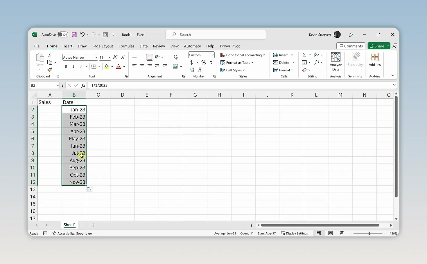
Next, enter the monthly cookie sales in A2 through A12. You can use your own sales figures to practice the same techniques. In our example, January starts at 1,000 cookies. New Year’s resolutions aren’t especially helpful to the cookie business.

4. Format and Organize Your Worksheet

Make numbers easier to read

A column of unformatted numbers can be difficult to scan. Thousands separators help you quickly distinguish a few thousand from tens of thousands.

1. Select the sales cells.
2. Open the Home tab.
3. In the number-formatting controls, choose the thousands-separator button, commonly shown as Comma Style.
4. Use Decrease Decimal until no decimal places remain.

We sell whole cookies here, so decimal places don’t add much value.

For more control, press Ctrl + 1 to open the Format Cells dialog. It provides options for numbers, dates, currency, and other cell formats. Keep this Excel keyboard shortcut reference handy as you learn.

AutoFit columns to their contents

Sometimes a number needs an explanation. Enter Notes in C1, then add a note in C2 explaining that New Year’s resolutions reduced January sales.

The text may extend into the empty cells to the right. To make it fit within column C, double-click the boundary between the C and D column headings. Excel automatically adjusts the column width to fit the contents.

To AutoFit several columns at once, select those columns and double-click a boundary between their headings. You can also select the entire worksheet using the triangle where the row and column headings meet, then AutoFit the columns. The same general approach works for row heights by double-clicking a boundary between row numbers.

Hide information without deleting it

Maybe management already knows why January sales were low. At least, I hope they do. We can hide the Notes column without throwing away the explanation.

• Hide a column: Right-click its column heading and choose Hide.
• Unhide a column: Select the columns on either side of the hidden column, right-click, and choose Unhide.
• Delete a column: Right-click its heading and choose Delete if you actually want to remove it.

Hiding keeps the data in the worksheet. It simply removes the column from the current display. You can hide and unhide rows in the same way.

Move the Date column before Sales

Our spreadsheet would make more sense with the date first and sales second.

1. Select the Date header and its monthly entries.
2. Hold Shift and point to the edge of the selection, not the fill handle.
3. When the move pointer appears, drag the selection to the left of Sales.
4. Release it at the insertion position.

Now Date is in column A and Sales is in column B. AutoFit the columns again if any values aren’t fully visible. We’ll use this arrangement for the formulas below.

5. Turn Your Data into an Excel Table

An Excel table does more than add a little color. It gives your data a defined structure and provides convenient tools for totals, sorting, and filtering.

1. Click a cell within your Date and Sales data.
2. Go to Insert > Table.
3. Check that Excel has selected the correct range.
4. Make sure My table has headers is checked.
5. Click OK.

Excel adds formatting, including banded rows that make the data easier to follow. Select the table to access the Table Design tab, where you can choose a different style.

Add a Total Row

On Table Design, turn on Total Row. In the bottom cell of the Sales column, open the dropdown and choose Sum.

Our January-through-November sales come to roughly 75,000 cookies. The cookie business is looking pretty good.

Insert a missing month

We still need December, which happens to be our strongest month. Apparently, calories become less concerning during the holidays.

1. Right-click the row number containing the Total Row, which is row 13 at this point.
2. Choose Insert to create space above the total.
3. Use November’s fill handle to extend the date series into December.
4. Enter December’s sales in the new Sales cell.

You can use the same right-click-and-insert approach on column headings when you need another column.

6. Highlight Highs and Lows with Conditional Formatting

The numbers tell us December was strong and January was weak, but we can make that difference easier to spot.

1. Select the monthly sales values, leaving out the header and total.
2. Go to Home > Conditional Formatting.
3. Choose Color Scales.
4. Select a scale that applies red to lower values and green to higher values.

Excel colors the cells based on their underlying values. Now the strongest and weakest months stand out immediately.

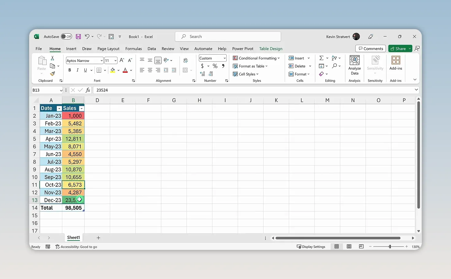
Color scales are only one option. Conditional formatting also includes data bars, icon sets, and custom rules. The main idea is that Excel applies the formatting according to the data, rather than requiring you to color each cell manually.

7. Calculate Totals with the Status Bar, Formulas, and Functions

Suppose we want to know how many cookies we sold in the first quarter, January through March. Excel gives us several ways to answer that question.

Get a quick answer from the status bar

Select the three sales cells, B2:B4, and look at the status bar along the bottom of the window. It can show the sum of the selected numbers without adding a calculation to your worksheet.

In our example, first-quarter sales are about 12,000 cookies.

Ask a question with Analyze Data

Another option is Home > Analyze Data. In the pane that opens, you can ask a question about your data, such as asking for total sales in Q1 as a table.

Excel returns an analysis without requiring you to write a formula. If this feature is available in your version, it’s a useful way to start exploring questions about your data.

Write a basic formula

To calculate the total yourself, select an empty cell outside the table and enter =B2+B3+B4, then press Enter.

The equals sign tells Excel that you’re entering a formula. The cell references tell it which values to use. You can type those references or click each cell as you build the formula.

Excel supports the familiar arithmetic operations:

• Addition: +
• Subtraction: -
• Multiplication: *
• Division: /

Use SUM to simplify the calculation

Clicking every cell is manageable for three months, but not especially convenient for a large range. A function is a built-in calculation that saves you that work.

Enter =SUM(B2:B4) in another empty cell and press Enter.

Here’s how it works:

• SUM is the function name.
• B2:B4 is the argument, or the range of cells the function should add.
• The colon means all cells from B2 through B4.
• The parentheses enclose the function’s argument.

You’ll get the same result as the addition formula, with much less typing. Open the Formulas tab to explore other functions and their categories. Microsoft’s Excel help and learning resources are also useful when you need more detail about a particular feature.

8. Sort and Filter Your Data

The dropdown arrows next to your table headers let you rearrange the data or focus on a smaller portion of it. You can toggle filtering controls from the Data tab, but we’ll leave them on.

Sort to rank your sales

Open the dropdown next to Sales and choose Sort Largest to Smallest. December moves to the top, and January lands at the bottom.

To return to chronological order, open the Date dropdown and choose Sort Oldest to Newest.

Filter to focus on the first quarter

1. Open the Date dropdown.
2. Deselect all dates.
3. Select only January, February, and March.
4. Click OK.

Only those months remain visible. Notice that the table’s Total Row updates to reflect the filtered data, giving us another way to calculate first-quarter sales.

When you’re finished, open the dropdown again and clear the filter to restore all months.

Sorting changes the order of your records. Filtering changes which records are displayed.

9. Create a Chart to See the Sales Trend

A worksheet is useful for finding an exact number. A chart makes the overall pattern easier to understand.

1. Click within your sales table.
2. Go to Insert > Recommended Charts.
3. Choose the recommended line chart.
4. Click OK.

A line chart works well here because we’re showing how sales change over time. It makes the monthly ups and downs clear, including that large jump in December.

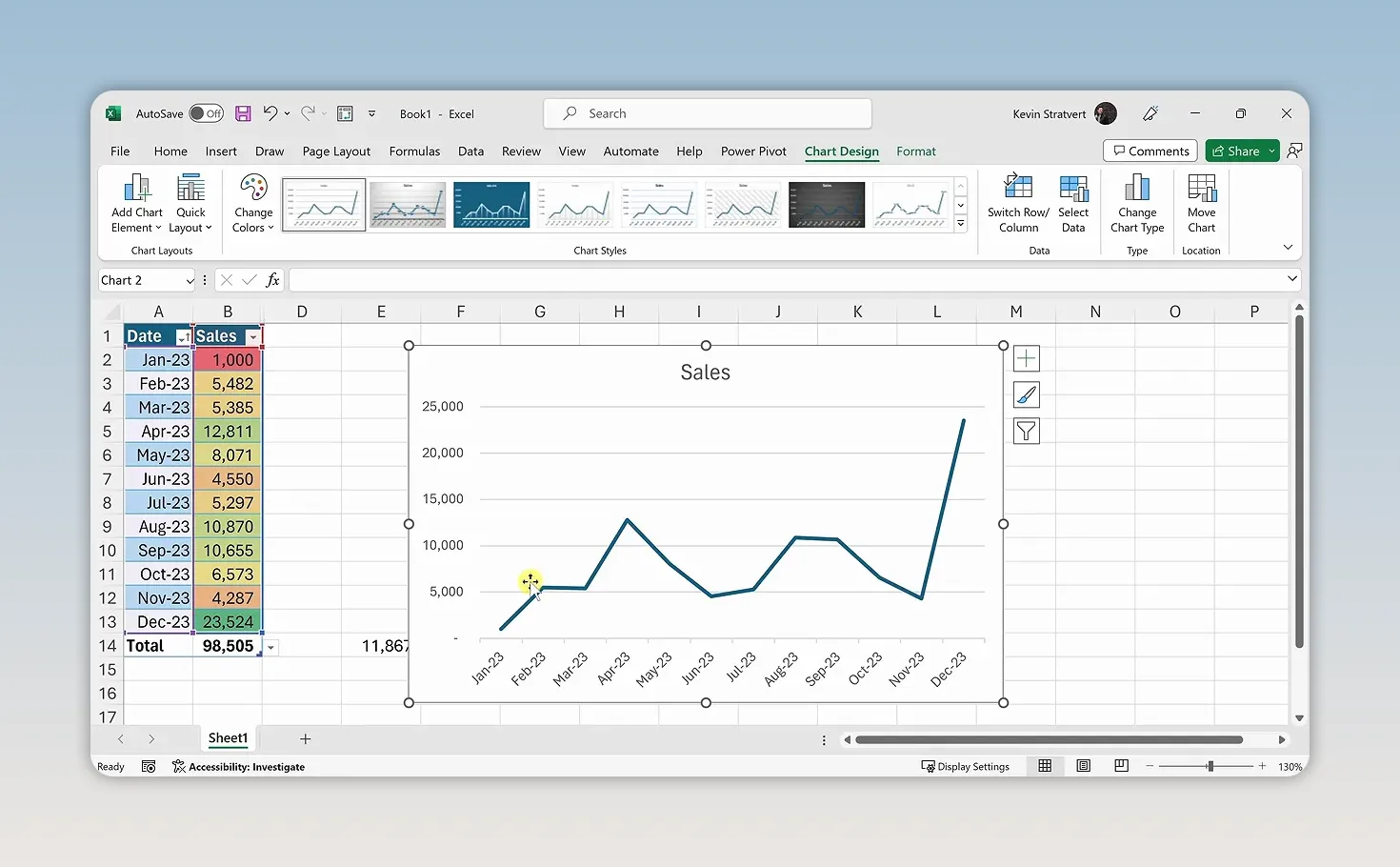
Select the chart to access tools for changing its style and appearance. You can also choose other chart types from the Insert tab rather than using a recommendation.

10. Analyze Data with a Pivot Table

Pivot tables are one of Excel’s most powerful analysis tools, and you can do a surprising amount just by dragging fields into different areas.

Create the pivot table

1. Click inside the original sales table.
2. Go to Insert > PivotTable.
3. Confirm the source data.
4. Choose New Worksheet.
5. Click OK.

Excel creates a new worksheet. Use the sheet tabs at the bottom to switch between the original data and the pivot table.

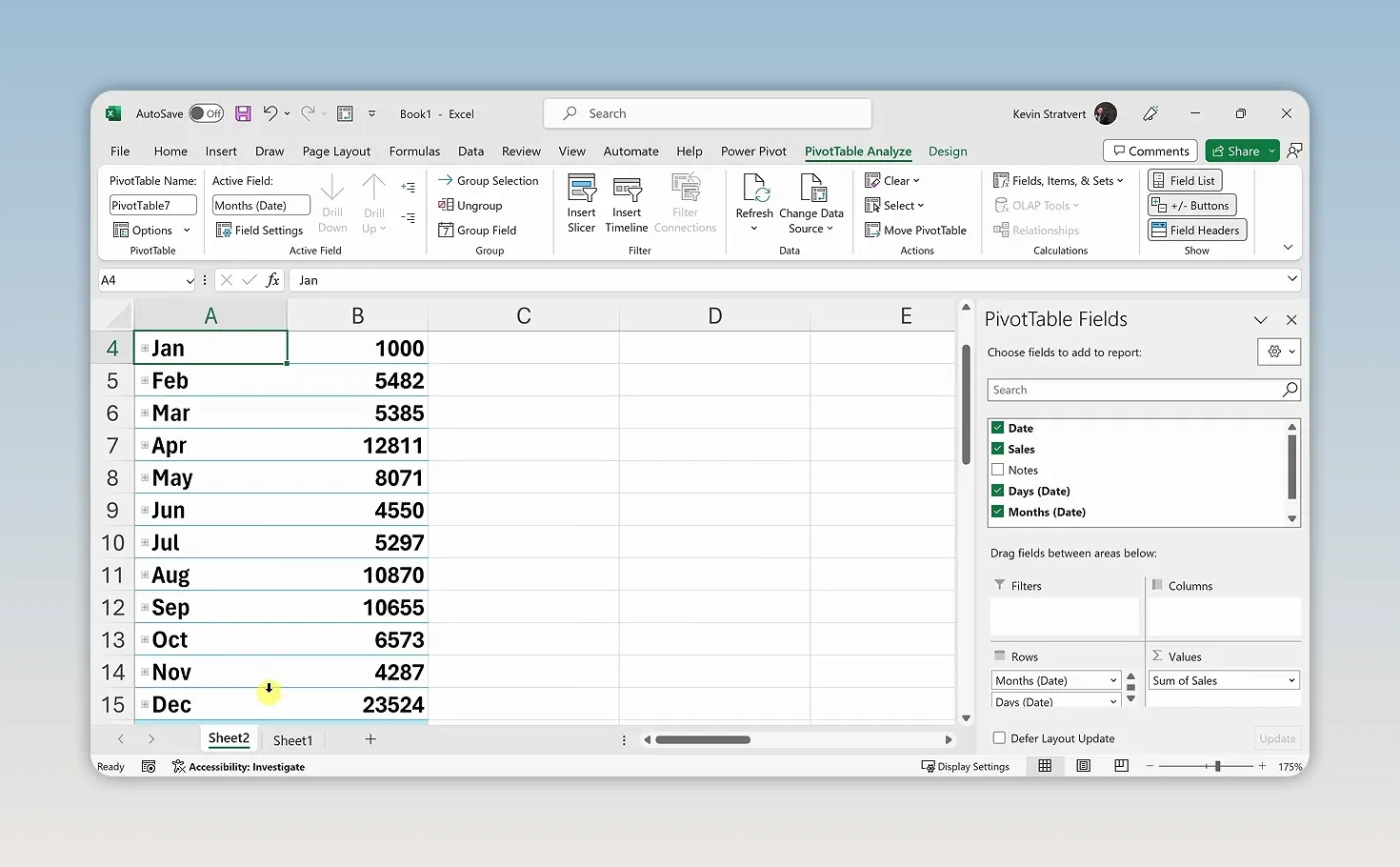
Click within the pivot table to display the PivotTable Fields pane. The fields correspond to columns in your source data, including Date and Sales.

Calculate total and average sales

Drag Sales into the Values area. This is where you put fields you want to calculate or summarize. Excel displays the sum of sales, which is nearly 100,000 cookies for the full year.

To change the calculation, right-click the result and choose Summarize Values By > Average. Now you can see average monthly sales, roughly 8,200 cookies. Use the same menu to switch back to Sum.

Explore Filters, Rows, and Columns

The placement of a field changes how the pivot table organizes your analysis:

• Filters: Drag Date here to filter the entire pivot table. Selecting January shows its 1,000 sales.
• Rows: Drag Date here to list months vertically, with their sales beside them.
• Columns: Move Date here to display the months horizontally across the worksheet.

To remove a field from an area, drag it out. You can then place it somewhere else to explore a different layout.

Show each month’s percentage of annual sales

A sales total answers how much we sold. A percentage answers how much each month contributed to the year.

1. Put Date in Rows and Sales in Values.
2. Right-click a sales value in the pivot table.
3. Choose Show Values As > % of Grand Total.

January accounts for about 1% of annual sales, while December contributes about 24%. That’s quite a difference, and it becomes clear without writing a separate percentage formula for every month.

For more practice with pivot tables and other analysis tools, my free Excel lesson playlist covers these topics in greater depth.

11. Share Your Workbook with Your Team

Once your analysis is ready, you can share the workbook directly from Excel.

1. Make sure the workbook is saved in OneDrive.
2. Click Share in the upper-right corner, then choose Share from the menu if prompted.
3. Enter or select the people you want to share it with.
4. Click Send.

You now have a workbook that does much more than store numbers. It organizes monthly sales, highlights strong and weak results, calculates totals, shows trends, and breaks down each month’s contribution to the year.

The best next step is to repeat these techniques with data you care about. Start with a small dataset, ask a useful question, and choose the Excel tool that helps answer it. That’s how you start building your data-analysis skills.

If you prefer a structured path through the fundamentals, my Excel for Beginners course walks through the essentials step by step.