How to Use Excel for Beginners in 10 Minutes

Does your resume say you know Excel, but you haven’t actually used it? We can fix that. You don’t need to memorize every button or learn hundreds of formulas to get started. A simple spreadsheet is enough to learn the basics.

We’ll build a monthly sales tracker for the Kevin Cookie Company. Along the way, you’ll enter and format data, turn it into an Excel table, highlight trends, create a chart, calculate totals, and explore your data with Copilot.

Table of Contents

• 1. Understand cells, rows, and columns
• 2. Build your first spreadsheet
• 3. Make the spreadsheet easier to read
• 4. Turn your data into an Excel table
• 5. Highlight trends with conditional formatting
• 6. Create a chart to visualize sales
• 7. Calculate Q4 sales with a formula
• 8. Use the SUM function to work faster
• 9. Sort and filter your data
• 10. Explore your data with Excel Copilot
• You have the foundation. Now build on it.

1. Understand cells, rows, and columns

The grid where you work in Excel is called a worksheet. Each box in that grid is a cell, and that’s where you enter information.

• Columns run vertically and have letters across the top: A, B, C, and so on.
• Rows run horizontally and have numbers down the left side.
• A cell address combines the column letter and row number.

For example, A1 is the cell in column A, row 1. D6 is in column D, row 6. These addresses become especially useful when you start calculating with your data.

2. Build your first spreadsheet

Instead of exploring every Excel feature in isolation, let’s give the worksheet a job: tracking how many cookies we sell each month.

1. Click cell A1, type Date, and press Tab to move to B1.
2. Type Sales in B1, then press Enter.
3. Click cell A2 and type January.

You could type the remaining months one at a time, but Excel can do that work for you.

Select A2 again and move your pointer over its bottom-right corner. When the pointer changes, click and drag down through A13. This little corner control is the fill handle. Excel recognizes the month sequence and fills in February through December.

Now enter the monthly sales in cells B2 through B13, pressing Enter after each number. To use the same example, enter these values:

• January: 1,200
• February: 1,800
• March: 2,400
• April: 3,200
• May: 4,100
• June: 5,000
• July: 6,200
• August: 6,800
• September: 5,900
• October: 7,200
• November: 9,500
• December: 14,500

Just like that, you have a working data set. It isn’t fancy yet, but everything we need is there.

3. Make the spreadsheet easier to read

Format the sales numbers

A column of numbers is easier to scan when thousands have separators. And since we’re counting cookies, we don’t need decimal places.

1. Select the sales values in B2:B13.
2. Open the Home tab.
3. In the number-formatting controls, click the comma-style button to add a thousands separator.
4. If Excel displays two decimal places, click Decrease Decimal twice.

Now a value such as 1200 displays as 1,200. Much easier to read.

Adjust the column width with AutoFit

Some month names may be cut off because column A is too narrow. To widen it manually, move your pointer to the boundary between the A and B column headings, then click and drag.

Here’s a quicker trick: double-click that boundary. Excel automatically fits the column width to its contents. No more missing letters in September.

4. Turn your data into an Excel table

An Excel table is more than a nice-looking range of cells. It adds useful tools for totals, sorting, and filtering, making it one of the best features to learn early.

1. Click any cell inside your data.
2. Choose Insert > Table, or use the Ctrl+T shortcut.
3. Check that Excel has selected the correct range: A1:B13.
4. Keep My table has headers selected because Date and Sales are your column headings.
5. Click OK.

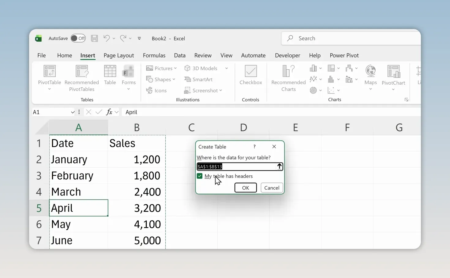
Excel applies table formatting and adds dropdown arrows to the headings. You’ll also see a Table Design tab when a cell inside the table is selected.

Add a Total Row

Click inside the table, open Table Design, and select Total Row. A new row appears at the bottom.

Click the sales cell in that row and use its dropdown to choose Sum. For this example, the annual total is 67,800 cookies. You can also choose another calculation, such as Average, but we’ll keep Sum.

Apparently, there really is something to this cookie business.

5. Highlight trends with conditional formatting

The numbers are readable now, but finding patterns still takes some effort. Conditional formatting adds visual cues so high and low values stand out immediately.

1. Select the monthly sales values in the table, leaving out the annual total.
2. Open Home > Conditional Formatting.
3. Point to Color Scales.
4. Choose the first color scale shown in the example.

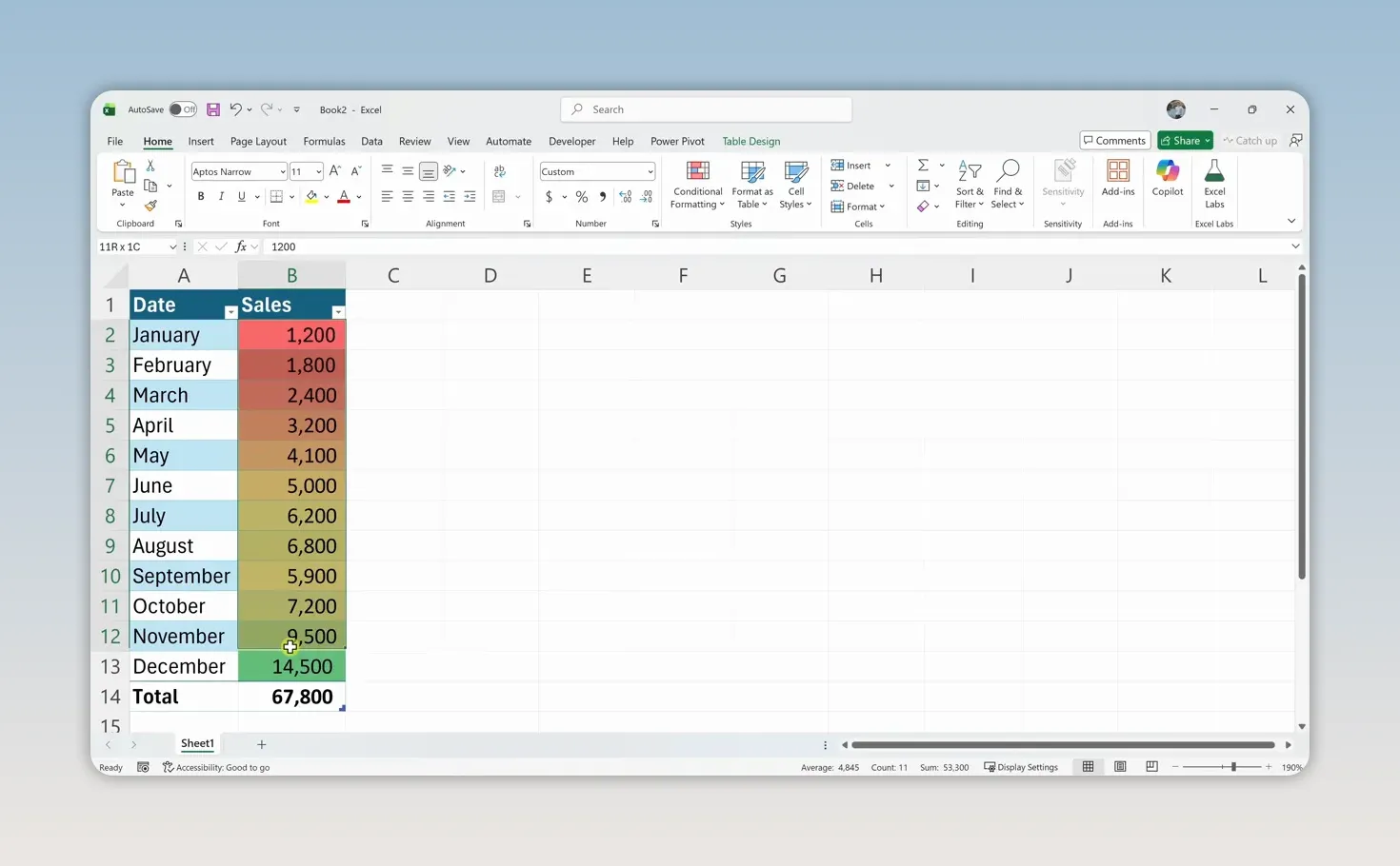
Lower sales appear toward the red end of the scale, while higher sales appear toward green. You can quickly see that sales generally increase as the year progresses, with the strongest results around the holidays.

6. Create a chart to visualize sales

A color scale helps you compare individual values. A chart makes the overall trend even easier to understand.

1. Select the month and sales data, including the headings but not the Total Row.
2. Open the Insert tab.
3. Choose Recommended Charts.
4. Select the line chart and click OK.

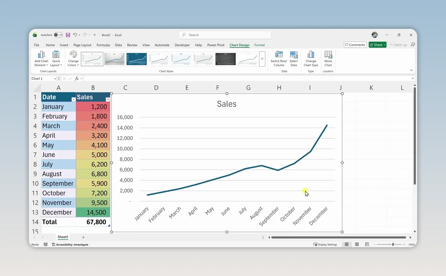
A line chart works well here because we’re showing sales over time. The upward trend and the sharp increase near the end of the year are much easier to spot than they are in a plain list of numbers.

7. Calculate Q4 sales with a formula

Now let’s answer a specific question: how many cookies did we sell in the final quarter of the year?

With the months still in January-to-December order, October, November, and December occupy cells B11:B13. Select those three sales cells and look at Excel’s status bar at the bottom of the window. It shows a sum of 31,200.

That’s handy for a quick check, but the result disappears from the status bar when you select something else. To keep it on the worksheet, create a formula.

1. Click A16 and type Q4:.
2. Click B16 and type =B11+B12+B13.
3. Press Enter.

You can also build the formula by typing an equals sign, clicking B11, typing a plus sign, clicking B12, adding another plus sign, and clicking B13.

The equals sign tells Excel you’re entering a formula. The cell references tell it which values to use. The result is 31,200, without pulling out a calculator.

8. Use the SUM function to work faster

Adding three cells individually is manageable. Adding a much longer list that way would get tedious. That’s where functions come in.

A function is a built-in calculation you can use inside a formula. One of the most common is SUM.

In the cell next to your first Q4 result, enter =SUM(B11:B13) and press Enter. You’ll get the same answer: 31,200.

• = starts the formula.
• SUM tells Excel to add values.
• B11:B13 is the argument, or input, supplied to the function.
• The colon means the range from B11 through B13, including the cells between them.

To build it with your mouse, type =SUM(, select the three sales cells, type the closing parenthesis, and press Enter.

The Formulas tab contains many more functions to explore. For a closer reference on this one, Microsoft’s SUM function guide explains its syntax and usage.

9. Sort and filter your data

The dropdown arrows in your table headings make it easy to reorganize the data or focus on just part of it.

Sort sales from largest to smallest

Open the dropdown in the Sales heading and choose Sort Largest to Smallest. December moves to the top with 14,500 sales, followed by November and October.

This answers a different question from the chronological chart: rather than asking how sales changed over time, you’re ranking the months by performance.

Filter to the final quarter

1. Open the dropdown in the Date heading.
2. Clear the selection of all months.
3. Select only October, November, and December.
4. Click OK.

Only those three months remain visible. Even better, the table’s Total Row automatically updates to show the total for the filtered results: 31,200.

To bring everything back, open the Date dropdown again and choose the option to clear the filter.

10. Explore your data with Excel Copilot

Excel also includes AI tools through Copilot. Rather than writing a formula, you can ask a question in everyday language.

Open the Home tab and select Copilot on the right side of the ribbon. In its side panel, enter a question such as What are my total sales? and submit it.

For our cookie sales example, Copilot returns 67,800, matching the annual total in the table.

You can also ask Copilot to create charts, summarize trends, or highlight insights in your data. It provides another way to explore a spreadsheet, especially when you’re still getting comfortable with formulas and Excel’s menus.

You have the foundation. Now build on it.

You’ve gone from a blank worksheet to a formatted sales tracker with a table, visual trends, a chart, and calculations. You also know how to rank results, filter to a specific period, and ask Copilot questions about your data.

Those are practical skills you can start using right away. The next step is to repeat the process with your own data, one useful spreadsheet at a time.