Excel Formulas and Functions Tutorial for Beginners

Excel formulas let you do much more than store numbers in a spreadsheet. You can add up a range of cells, calculate an average, combine names, make decisions, and look up information automatically.

The nice thing is that you do not need to learn everything at once. Start with a few basic calculations, and the same patterns carry over to more powerful functions like IF, VLOOKUP, and SUMIF.

Table of Contents

• How to Enter a Formula in Excel
• Add, Subtract, Multiply, and Divide
• Use SUM to Add a Range of Cells
• Find the Smallest and Largest Values with MIN and MAX
• Count Cells with COUNT and COUNTA
• Calculate the Average and Median
• Combine Text with CONCAT
• Add Logic with IF
• Count Matching Values with COUNTIF
• Look Up Information with VLOOKUP
• Add Only Matching Values with SUMIF
• Get the Current Date and Time with NOW
• Start with the Pattern, Then Build from There

How to Enter a Formula in Excel

Start your formula with an equal sign. That tells Excel you want it to calculate something.

1. Click the cell where you want the result to appear.
2. Type =, followed by your calculation.
3. Press Enter.

For example, enter =1+1, and Excel displays 2. Select that cell again, and you can see the underlying formula in the formula bar above the worksheet.

You can type numbers directly into a formula, but you can also refer to cells that already contain numbers. A reference like B1 means column B, row 1.

If B1 contains 1 and C1 contains 1, enter =B1+C1 in another cell. You get the same result, but now the formula uses the values in your worksheet. Change those values, and the result updates automatically.

You do not have to type every cell reference, either. While building a formula, click a cell to insert its reference. For many calculations, that is the easier option.

Add, Subtract, Multiply, and Divide

The four basic arithmetic operations all follow the same pattern. Start with an equal sign, select or type the first value, enter an operator, and select or type the second value.

• Add: =B1+C1. If both cells contain 1, the result is 2.
• Subtract: =B2-C2. If B2 contains 2 and C2 contains 1, the result is 1. No big surprise there.
• Multiply: =B3*C3. If both cells contain 2, the result is 4.
• Divide: =B4/C4. If B4 contains 4 and C4 contains 2, the result is 2.

Two symbols are worth remembering: multiplication uses an asterisk, not the letter X, and division uses a forward slash.

These formulas work well for a couple of values. But what if you want to add an entire block of numbers? You probably do not want to click each cell and keep typing plus signs. That is where functions come in.

Use SUM to Add a Range of Cells

A function is a built-in calculation you can use inside a formula. SUM, for example, adds numbers for you.

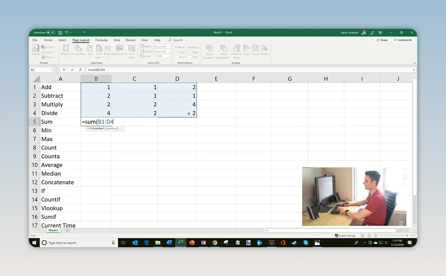
To add all the values in B1 through D4, enter =SUM(B1:D4) in a cell outside that range.

Here is how to build it with your mouse:

1. Type =SUM(.
2. Click and drag to select B1 through D4.
3. Type the closing parenthesis, ).
4. Press Enter.

The colon in B1:D4 means the whole rectangular range between those two cells, including both endpoints. With the arithmetic examples above and their results in column D, that block adds up to 24.

You can also give SUM separate values or references, separated by commas, such as =SUM(B1,C1,D1). For one continuous block of cells, selecting a range is much quicker.

Get Help with the Insert Function Button

If typing function names and parentheses feels a little unfamiliar, click the Insert Function button, labeled fx, beside the formula bar.

Search for or select SUM, then use the Function Arguments dialog to select the numbers you want to add. Click OK, and Excel builds the formula for you.

This is another way to enter the same calculation, and it gives you some guidance as you go.

Find the Smallest and Largest Values with MIN and MAX

Once you know how to use SUM, several other functions should feel familiar. You still enter the function name, open a parenthesis, select your cells, and close the parenthesis.

• Smallest value: =MIN(B1:D4)
• Largest value: =MAX(B1:D4)

In the original block of arithmetic examples, MIN returns 1 and MAX returns 4.

Now change an input value to 10. MAX updates to reflect the new largest value. Change an input to 0, and MIN picks up the new minimum.

You are creating a calculation connected to your data, not just typing an answer. That connection is what makes formulas useful when your numbers change.

Count Cells with COUNT and COUNTA

COUNT and COUNTA sound similar, but they answer different questions.

COUNT: How Many Cells Contain Numbers?

Enter =COUNT(B1:D4) to count the cells in that range that contain numbers.

Our four-row, three-column example contains 12 numeric cells, so COUNT returns 12.

If you expand the selection to include blank cells, the result stays the same. Blank cells do not add to the count. Text does not add to it, either.

COUNTA: How Many Cells Are Not Empty?

Use COUNTA when you want to count cells containing values, including text.

For example, =COUNTA(B1:G4) counts the nonempty cells in that larger range. If it contains the same 12 numeric cells plus the name Kevin, COUNTA returns 13. Add Seattle to another blank cell within the range, and it returns 14.

COUNT still returns 12 for that same selection because the two added entries are text.

The distinction is simple: COUNT counts numeric cells; COUNTA counts nonempty cells.

Calculate the Average and Median

AVERAGE and MEDIAN both help describe a group of numbers, but they do not calculate the same thing.

Consider these four salaries:

• $100,000
• $15,000
• $25,000
• $30,000

You can apply a currency format to make them easier to recognize as dollar amounts. The functions still work with the underlying numbers.

AVERAGE: Calculate the Arithmetic Mean

If those salaries are in D10:G10, enter =AVERAGE(D10:G10).

The result is $42,500. Excel adds the four salaries and divides by four.

Notice that the $100,000 salary pulls the average upward. Three of the four salaries are below the calculated average.

MEDIAN: Find the Middle Value

For the same salaries, enter =MEDIAN(D10:G10).

Imagine arranging the values from smallest to largest: $15,000, $25,000, $30,000, and $100,000. With four values, the middle lies between $25,000 and $30,000. Excel averages those two middle values, giving a median of $27,500.

If you add another $30,000 salary and extend the formula to include it, the median becomes $30,000, the middle value of the five salaries.

That explains why an average and a median can look quite different. The average uses every amount in its calculation, while the median identifies the center of the ordered values.

Combine Text with CONCAT

Formulas are not just for numbers. You can also join text, which is called concatenation. The word sounds complicated, but the task is straightforward.

Suppose D12 contains Kevin and E12 contains Stratvert. Enter =CONCAT(D12,E12) to join the two values.

The result is KevinStratvert. It works, but it needs a space.

You can put a space in another cell, such as F12, and include it between the two names: =CONCAT(D12,F12,E12).

Or include the space directly in the formula: =CONCAT(D12," ",E12). Either way, the result is Kevin Stratvert.

Commas separate the pieces you want to combine, and their order determines the order of the final text. If your older version of Excel does not recognize CONCAT, use CONCATENATE for this same example.

Add Logic with IF

The IF function lets Excel return one result when a condition is true and a different result when it is false.

Suppose D13 contains the word smile. Enter =IF(D13="smile","yay","boo") in another cell.

The formula has three parts:

1. Logical test: Does D13 equal "smile"?
2. Value if true: Return "yay".
3. Value if false: Return "boo".

With smile in D13, the result is yay. Change it to frown, and the result becomes boo.

Put text values inside double quotation marks when entering them directly into a formula. Also notice that this example tests whether the cell equals the word smile, rather than whether smile appears somewhere inside a longer sentence.

Count Matching Values with COUNTIF

COUNT counts numeric cells. COUNTIF goes a step further: it counts cells that meet a condition.

To count how many cells in B1:D4 contain the number 10, enter =COUNTIF(B1:D4,10).

It takes two arguments:

• Range: The cells Excel should check.
• Criteria: The value or condition to look for.

If only one cell in the selected range contains 10, the result is 1. You do not need to inspect and count the matches yourself.

Look Up Information with VLOOKUP

VLOOKUP finds a value in the first column of a selected range, then returns information from another column in the same row.

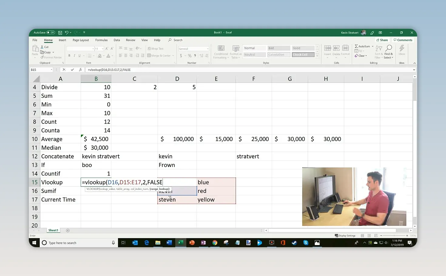
For a simple example, enter names in D15:D17 and their favorite colors in E15:E17:

• Kevin: red
• Alex: blue
• Steven: yellow

To find Kevin's favorite color, enter =VLOOKUP("Kevin",D15:E17,2,FALSE).

Here is what each argument does:

1. "Kevin": The value to find.
2. D15:E17: The range containing the names and colors.
3. 2: Return the value from the second column of that range.
4. FALSE: Require an exact match.

The result is red. Excel finds Kevin in the first column and returns the color beside his name.

For this name lookup, use an exact match. Approximate matching is not a way to find a similar spelling or a partially matching name. It follows lookup-order rules and is intended for different situations. Microsoft's VLOOKUP documentation explains the matching options in more detail.

For a more detailed walkthrough, my VLOOKUP and HLOOKUP tutorial covers both lookup functions.

Add Only Matching Values with SUMIF

SUMIF combines a condition with addition. Instead of counting matching cells, it adds the values associated with those matches.

Suppose D16:F16 contains the names Alex, Kevin, and Kevin, and D17:F17 contains their associated values: 5, 10, and 5.

To add only the values associated with Kevin, enter =SUMIF(D16:F16,"Kevin",D17:F17).

The three arguments are:

• Range: D16:F16, the cells containing the names to check.
• Criteria: "Kevin", the name to match.
• Sum range: D17:F17, the corresponding numbers to add.

There are two Kevin entries, associated with 10 and 5, so the result is 15. The 5 associated with Alex is excluded.

The important part is keeping the names and their corresponding values aligned. Excel checks one position in the criteria range and adds the value from the corresponding position in the sum range.

Get the Current Date and Time with NOW

For a simple finish, enter =NOW() to return the current date and time.

This function does not need any arguments, but it still needs both the opening and closing parentheses.

Unlike a date and time you type manually, NOW is a formula. It updates when Excel recalculates, rather than acting as a permanent timestamp.

Start with the Pattern, Then Build from There

Most of these functions follow a familiar rhythm: type an equal sign, enter the function name, open the parentheses, select the relevant cells, and close the parentheses.

Start with basic arithmetic and SUM. Then try counting cells, comparing AVERAGE with MEDIAN, and adding a condition with IF. From there, COUNTIF, VLOOKUP, and SUMIF give you ways to answer more specific questions about your data.

You do not need to memorize every function. Knowing what you want to calculate, and which cells contain the information, gets you a long way.

Made with VideoToBlog using Excel Formulas and Functions Tutorial