Excel Pivot Table Tutorial: A Step-by-Step Guide for Beginners

How many cars do I have by make? Which vehicles offer the most profit? What percentage of my inventory is black or silver?

You could answer those questions with filters and a collection of formulas. But there’s a much faster way: PivotTables in Microsoft Excel. Drag a few fields into place, and Excel can count, total, average, and visualize your data without requiring a separate formula for every question.

For a practical example, I’m going to pretend I run a used car dealership. We’ll use the same inventory to build several different reports, calculate expected profit, and create a chart that changes along with the analysis.

Table of Contents

• Start with the Car Inventory Data
• 1. Insert a PivotTable in Excel
• 2. Understand Filters, Rows, Columns, and Values
• 3. Add a Calculated Field for Expected Profit
• 4. Use Value Field Settings to Calculate Averages
• 5. Show Values as a Percentage of the Total
• 6. Create a PivotChart
• 7. Use Defer Layout Update for Larger Data Sets
• 8. Work with PivotTables in Excel for the Web
• Get Comfortable by Rearranging the Fields

Start with the Car Inventory Data

You can follow along using the sample car inventory workbook. It contains 24 vehicles, with one vehicle per row and fields for:

• Make: Chevrolet, Dodge, Ford, Honda, Nissan, or Toyota.
• Model: The specific vehicle model, such as an Accord, Camry, or Altima.
• Color: The vehicle’s color.
• Mileage: How many miles the vehicle has traveled.
• Price: What I expect to sell the vehicle for.
• Cost: What I paid for the vehicle.

The distinction between price and cost is important. If I paid $3,000 for a car and expect to sell it for $4,000, that leaves $1,000 in expected profit. Hey, I have to make a living, too.

The examples use desktop Excel with Microsoft 365. The same basic PivotTable workflow also applies to versions such as Excel 2019, 2016, and 2013, although the ribbon and menu labels may look a little different.

1. Insert a PivotTable in Excel

First, click a cell within the inventory data. Then open the Insert tab on the ribbon.

You have two useful starting points:

• Recommended PivotTables: Excel suggests report layouts based on your data and provides previews. In this inventory, one suggestion summarizes mileage by make.
• PivotTable: Start with a blank report and choose exactly how to organize it.

Recommended PivotTables can save time, but building one from scratch makes it much easier to understand how the pieces work.

1. Select Insert > PivotTable.
2. Check the source data range. Excel automatically selects the inventory in this example, but you can change the range if necessary.
3. Choose New Worksheet to give the report its own sheet. You can also place it on an existing worksheet.
4. Click OK.

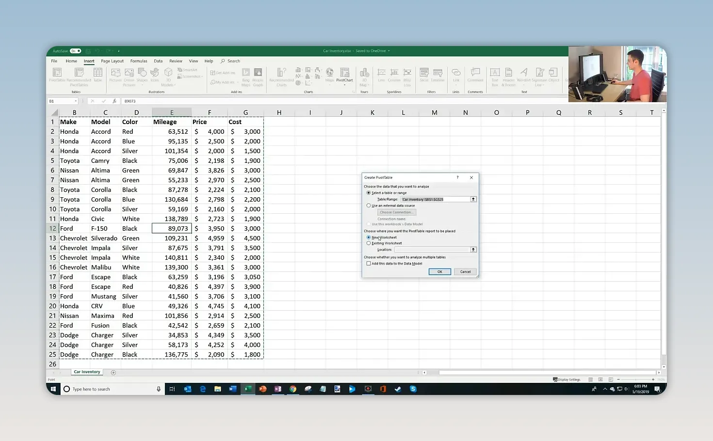
Excel creates an empty PivotTable and opens the PivotTable Fields pane on the right. It may look a little intimidating at first, but you only need to understand four areas.

2. Understand Filters, Rows, Columns, and Values

The field list contains the column headings from your source data. You build the report by dragging those fields into the boxes below the list.

• Filters: Restrict the report to selected items from a field.
• Rows: Arrange categories vertically down the worksheet.
• Columns: Arrange categories horizontally across the worksheet.
• Values: Perform the calculation, such as a count, sum, or average.

A useful way to think about it is this: Rows and Columns determine how you group the data; Values determines what you calculate.

Count Vehicles by Make, Model, and Color

My first question is straightforward: what does my inventory look like?

1. Drag Make into Rows.
2. Drag Model into Rows, underneath Make.
3. Drag Color into Columns.
4. Drag Make into Values as well.

Make can appear in both Rows and Values because those areas serve different purposes. In Rows, it creates the groups. In Values, Excel counts the text entries, producing Count of Make.

You now have makes down the left, models nested under each make, colors across the top, and vehicle counts where they intersect.

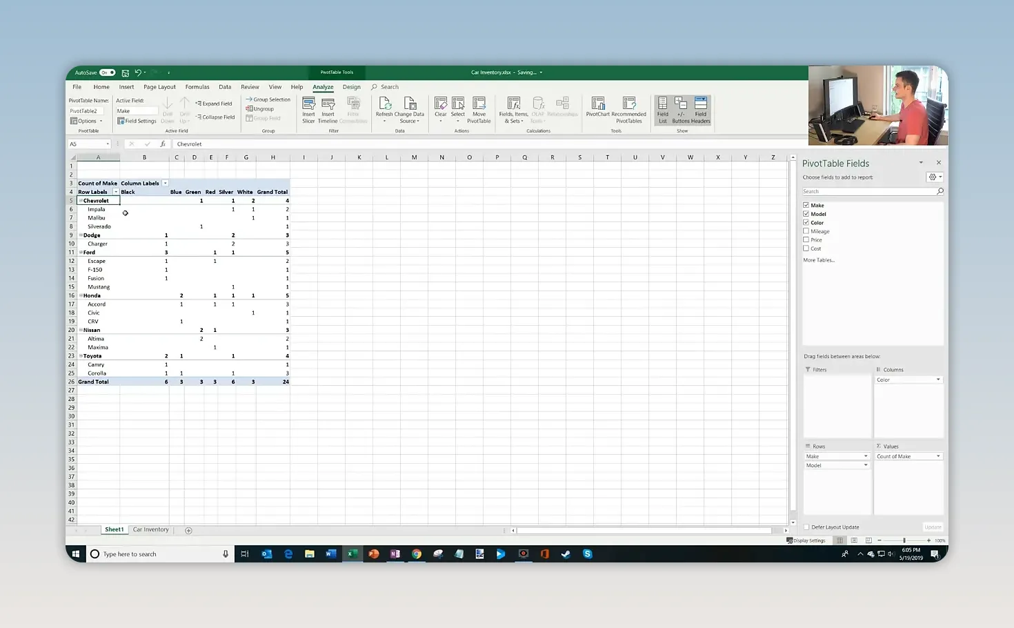
You can expand a make to see its individual models or collapse it to focus on the make-level totals. The ribbon also includes controls to expand or collapse an entire field.

For example, collapsing the model detail shows that Chevrolet has:

• 1 green vehicle.
• 1 silver vehicle.
• 2 white vehicles.
• 4 vehicles in total.

Expand Chevrolet again, and you can see which models account for those colors. No separate counting formulas required.

3. Add a Calculated Field for Expected Profit

Next, I want to know how much profit I expect to make from each make of vehicle.

You don’t need to create another PivotTable to answer a new question. Drag fields out of the layout areas to remove them, then arrange the fields you need for the next report.

Set up the report like this:

• Rows: Make.
• Values: Price and Cost, both summarized by Sum.
• Columns: Remove Color so the results are no longer split by vehicle color.

You can also keep Count of Make in Values if you want the number of vehicles beside the financial totals.

For the four Chevrolets, the expected selling prices total $14,500, and the purchase costs total $13,000. To calculate the difference within the PivotTable, add a calculated field.

1. Click inside the PivotTable.
2. Open the Analyze or PivotTable Analyze tab.
3. Select Fields, Items & Sets > Calculated Field.
4. Enter a name, such as Expected Profit.
5. Enter the formula =Price-Cost. You can select each field in the dialog and use Insert Field rather than typing its name.
6. Click Add, then OK.

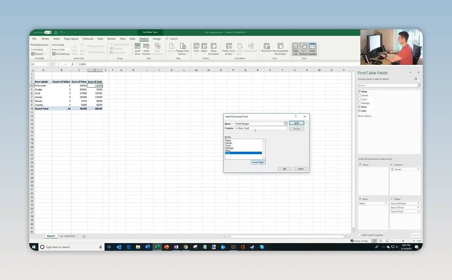
The calculated field appears in the report alongside the other values. For Chevrolet, the result is $1,500 in expected profit.

This calculation gives a dollar amount, not a profit margin percentage. It also uses the expected selling price, so it represents what I anticipate earning if the vehicles sell at those prices.

Sort to Find the Largest Profit

I could read through every result to find the largest one, but sorting makes that much easier:

1. Right-click a number in the Expected Profit column.
2. Select Sort.
3. Choose Sort Largest to Smallest.

Honda moves to the top. Across the five Honda vehicles, I expect to make about $3,468, the largest total expected profit by make in this inventory.

4. Use Value Field Settings to Calculate Averages

A total tells me how much money I spent on a make. But what if I want to know the average amount I paid per vehicle?

Keep Make in Rows and Cost in Values. Remove the other value fields if you want a simpler report.

1. Open the dropdown beside Sum of Cost in the Values area.
2. Select Value Field Settings.
3. Under the calculation options, select Average.
4. Click OK.

The report changes from total purchase cost to average purchase cost. In the sample inventory:

• Chevrolet: I paid an average of $3,250 per vehicle.
• Honda: I paid an average of $2,500 per vehicle.

Apply a currency format to make those amounts easier to read.

Value Field Settings controls how Excel summarizes the records. Sum, Count, and Average answer different questions, and you can switch between them without writing new formulas.

5. Show Values as a Percentage of the Total

Now I want to understand my inventory by color. I know black and silver are popular, but how much of my lot do they actually represent?

Rearrange the report again:

1. Remove Make from Rows and Cost from Values.
2. Drag Color into Rows.
3. Drag Color into Values to create a count.
4. If the cells retain currency formatting from the previous report, change them back to a regular number format.
5. Sort the counts from largest to smallest.

The 24 vehicles break down into six black cars, six silver cars, and three each of white, blue, red, and green.

To turn those counts into percentages:

1. Right-click one of the counts.
2. Select Show Values As.
3. Choose % of Column Total.

Silver now shows 25%, and black also shows 25%. Each of the other four colors accounts for 12.5%.

There’s an important distinction here:

• Value Field Settings chooses the underlying summary calculation, such as Count or Average.
• Show Values As changes how that summary is displayed, such as a percentage of the column total.

In this case, Excel still counts the vehicles. It simply expresses each count as a share of the total.

6. Create a PivotChart

A numerical report is useful, but sometimes a chart makes the pattern much easier to recognize.

For this example, return the color summary to counts by choosing Show Values As > No Calculation. Then create a column chart:

1. Click inside the PivotTable.
2. Open Analyze or PivotTable Analyze.
3. Select PivotChart.
4. Choose a Column chart and click OK.

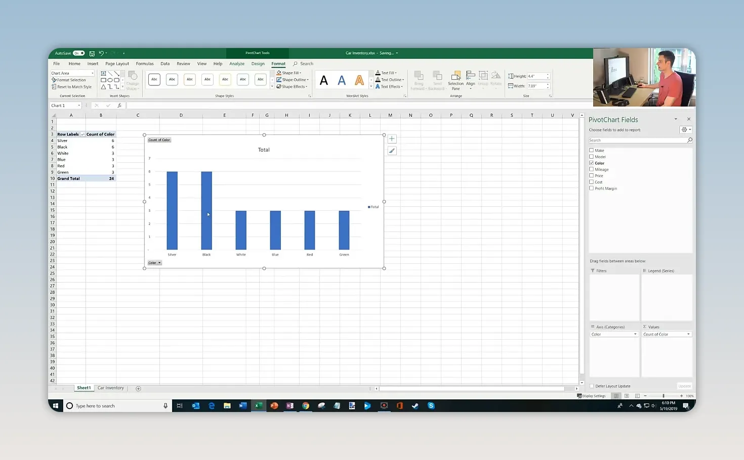
The chart shows black and silver at six vehicles each, with the remaining colors at three each.

The particularly useful part is that the PivotChart is connected to the PivotTable. When you add, remove, or rearrange fields, the chart updates to reflect the new report layout. You can explore a different breakdown without rebuilding the chart from scratch.

7. Use Defer Layout Update for Larger Data Sets

At the bottom of the Fields pane, you may notice a checkbox labeled Defer Layout Update.

Normally, each time you drag a field into or out of the layout, Excel recalculates the report. That’s convenient with 24 cars, but larger data sets can take more time to process.

Defer Layout Update lets you make several layout changes before asking Excel to apply them:

1. Check Defer Layout Update.
2. Add, remove, or rearrange the fields you need.
3. Click Update when the layout is ready.

Until you click Update, the PivotTable and connected chart keep their previous layout. This helps avoid waiting through a recalculation after every individual field change.

8. Work with PivotTables in Excel for the Web

You can also work with PivotTables in Excel for the web, which is available to use for free with a Microsoft account.

Sign in at Office.com and open the workbook. In this example, the file is stored in OneDrive, so the saved desktop changes are also available when I open it in the browser.

The inventory data, PivotTable, and chart are all there. You can select the sheet containing the report and use the field controls to rearrange the analysis. You can also start from the source data and use Insert > PivotTable to create a report in the browser.

That gives you a convenient way to continue working with the same workbook on the desktop or on the web.

Get Comfortable by Rearranging the Fields

The best way to learn PivotTables is to start with a question and experiment with the field placement.

Want to know how many vehicles you have? Put a text field in Values and count it. Want to compare purchase costs? Group by Make and summarize Cost. Want a share of inventory? Show the counts as a percentage of the total.

With one set of data, you’ve counted inventory, explored model and color detail, calculated expected profit, ranked results, compared average costs, and built a connected chart. Once those four layout areas make sense, PivotTables become a very approachable way to understand your data and make decisions from it.

Made with VideoToBlog using Pivot Table Excel Tutorial