How to Use Microsoft Power Query in Excel

If you spend more time cleaning up data than analyzing it, Power Query can take a lot of that repetitive work off your plate. It connects to your data, helps you reshape it, and remembers the changes so you can apply them again when new data arrives. Best of all, you can build this process without writing code.

Think about a recurring sales report. Every month, you find the latest file, remove unnecessary columns, split a few fields, add calculations, and finally get to the analysis. With Power Query, you define those cleanup steps once. The next time you receive a file, you refresh the query instead of repeating the work.

Power Query is available in both Microsoft Excel and Power BI. Here, I’ll use Excel and order data from the Kevin Cookie Company to build a complete workflow: combine files, clean the data, calculate profit and shipping time, and create an analysis that can include additional years.

Table of Contents

• Start with the Data You Want to Clean
• Find Power Query and Connect to a Folder
• Combine the Workbooks Before Loading Them
• Get Comfortable with the Power Query Editor
• Clean and Transform the Order Data
• Review and Adjust Applied Steps
• Close and Load the Cleaned Data into Excel
• Analyze Profit with a PivotTable and PivotChart
• Bring in New Files with Refresh All

Start with the Data You Want to Clean

At the Kevin Cookie Company, I have three Excel workbooks containing order data for 2017, 2018, and 2019. Another workbook for 2020 will arrive later. All of these files belong in the same folder.

Each workbook contains an Order Data worksheet with fields such as order ID, customer, cookies shipped, revenue, cost, order date, ship date, and order status.

The data needs a little help before it is ready for analysis:

• The customer ID and customer name are combined in one column.
• Cookies shipped is displayed as currency in the source workbook, even though it represents a unit count.
• There is no profit column.
• There is no calculation showing how many days each order took to ship.
• Promotional orders need to be excluded from the analysis.

They’re paying me to analyze cookie orders, but manually fixing all of this every time a file arrives doesn’t leave much time for analysis. That’s exactly the kind of task Power Query is good at.

You can use the sample workbooks to follow along. Keep the first three years together in a folder, and save the 2020 workbook for the refresh step.

Find Power Query and Connect to a Folder

In current Windows versions of Excel, open the Data tab. Power Query’s tools appear in the Get & Transform Data group.

Excel 2010 and Excel 2013 used a separate Power Query add-in. If you are working with one of those older versions, the Power Query add-in download page provides the relevant information.

Select Get Data to explore the available connections. Power Query can connect to a wide range of sources, including Excel workbooks, text files, PDFs, databases, and Azure services. The available connectors depend on your product and version. Microsoft’s Power Query overview provides more background on how it connects to and transforms data.

For this example, we want a connection to a folder rather than to one individual workbook. That way, the same query can pick up another year’s file later.

1. Go to Data > Get Data > From File > From Folder.
2. Paste the folder path, or select Browse to locate it.
3. Select OK.
4. Check the file list to confirm that Excel found the 2017, 2018, and 2019 workbooks.

Combine the Workbooks Before Loading Them

The folder preview offers several choices. The important distinction is whether you want to load the data immediately or make changes first.

• Load brings the data into Excel without first opening the editor for cleanup.
• Transform Data opens the Power Query Editor so you can modify the data.
• Combine & Transform Data combines the contents of multiple files and opens the editor.
• Combine & Load combines the files and loads the result without first stopping in the editor.

Since we have multiple workbooks and several changes to make, select Combine & Transform Data from the Combine menu.

In the Combine Files dialog, Power Query uses a sample file to identify which content to extract. The first file, containing the 2017 data, works for this example.

1. Leave Sample File set to the first file.
2. Select the Order Data worksheet.
3. Check the preview to confirm that it contains the expected order information.
4. Select OK.

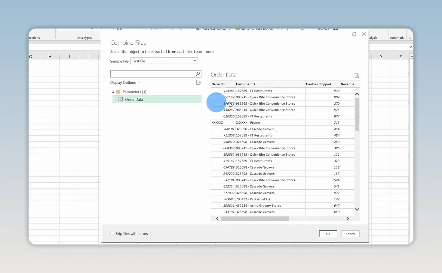
All of these workbooks have a worksheet with the same name and the same basic structure. That consistency allows Power Query to extract the corresponding data from each file.

Get Comfortable with the Power Query Editor

The editor might look a little intimidating at first, but there are just a few main areas to understand.

• Queries on the left: The folder-combine process creates helper queries, including a sample-file transformation, along with the final combined query. We’ll make the following changes in the final combined query.
• Data preview in the center: This shows the data as it looks at the selected stage of the query.
• Ribbon across the top: This contains tools for removing columns, splitting text, adding calculations, changing types, and more.
• Query Settings on the right: This includes the query name and the Applied Steps list.

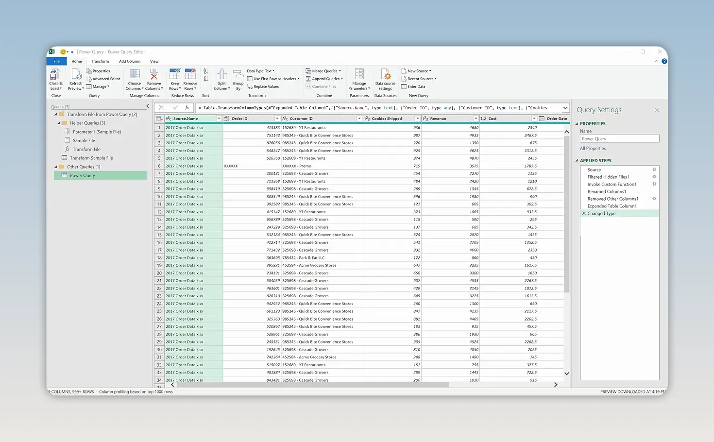
Applied Steps is the key to the automation. Each transformation becomes a saved step. It’s a little like recording a macro: Power Query remembers the sequence and runs it again when you refresh.

The preview in this example is limited to the top 1,000 rows. That does not mean the transformations only affect those rows. When you load or refresh the query, the steps apply to the full dataset.

Clean and Transform the Order Data

1. Remove the source filename column

The combined query includes a Source.Name column identifying the workbook each row came from. That can be useful, but I don’t need it for this analysis.

Right-click the Source.Name column header and select Remove.

2. Filter out promotional orders

Some rows use XXXXXX as the order ID. At the Kevin Cookie Company, these represent free cookies sent to events or used for promotions. They belong in the order records, but I don’t want them included in this particular sales analysis.

1. Open the filter menu on Order ID.
2. Find XXXXXX in the list.
3. Clear its checkbox and select OK.

This adds a filtering step to the query. The same exclusion will apply when additional data is brought in.

3. Split customer ID from customer name

The customer column contains two separate pieces of information joined by a space, a hyphen, and another space. We can use that separator, called a delimiter, to split the column.

1. Select the combined customer column.
2. Right-click its header and choose Split Column > By Delimiter.
3. Choose a custom delimiter and enter space + hyphen + space.
4. Select OK.
5. Double-click the resulting column headers and rename them Customer ID and Customer Name.

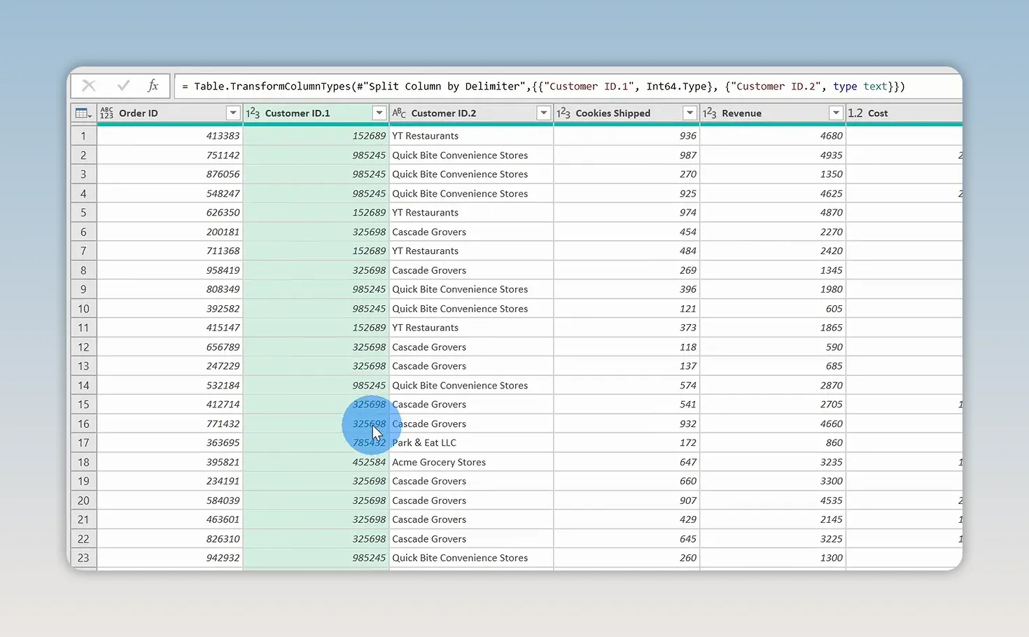
Including the spaces in the delimiter makes the split match the separator between the identifier and the name, rather than treating every hyphen as a separator.

Also notice that the Cookies Shipped values appear as numbers in the editor rather than carrying over the source worksheet’s dollar-sign formatting. A cookie count is a quantity, not a monetary amount. Revenue, cost, and profit are the fields that should use a currency data type.

4. Add a profit column

Profit is revenue minus cost. You can create that calculation directly from the ribbon without typing a formula.

1. Select the Revenue column first.
2. Hold Ctrl and select the Cost column.
3. Open Add Column > Standard > Subtract.
4. Rename the new Subtraction column to Profit.
5. Drag Profit so it sits immediately after Cost.

Selection order matters: we want revenue minus cost, not cost minus revenue.

Use Add Column here because we want to keep the original revenue and cost fields and create an additional result.

To assign the monetary data type, select Revenue, Cost, and Profit, then right-click and choose Change Type > Currency. The icons next to the column names indicate their data types.

5. Calculate days to ship

Next, I want to know how long orders sit between being placed and leaving the warehouse. We already have both dates, so we just need their difference.

1. Select Ship Date first.
2. Hold Ctrl and select Order Date.
3. Open Add Column > Date > Subtract Days.
4. Rename the result Days to Ship.
5. Drag the new column next to the order and shipping dates.

The calculation is Ship Date minus Order Date. Selecting the dates in that order gives us the elapsed shipping preparation time.

Some orders show five days just to get cookies out of the warehouse. That’s a conversation I need to have with the warehouse team. More importantly, this new column gives me something concrete to analyze instead of relying on a vague impression that shipping is slow.

Review and Adjust Applied Steps

As you make changes, Power Query builds a history in the Applied Steps pane. You can use that history to review how the data was shaped and adjust the process.

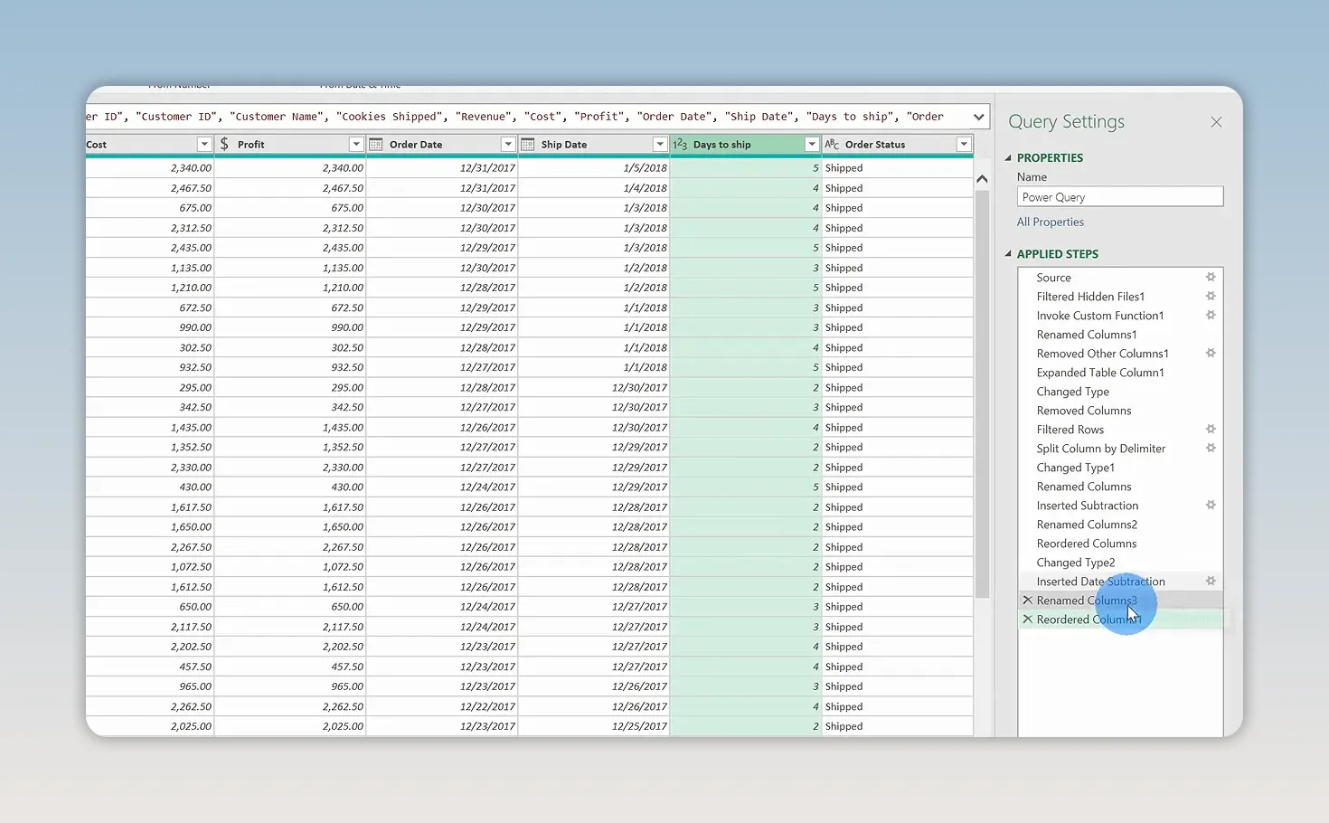
For example, suppose I right-click Order Status and remove it, then decide I actually want to keep it. Power Query adds a new removal step. Clicking the X beside that step removes the transformation and restores the column.

You can also move a step earlier or later in the sequence when appropriate. Keep the dependencies in mind: a calculation needs its input columns to exist at the point where it runs.

The goal isn’t just a clean preview. You’re building a repeatable set of instructions for the next batch of data.

Close and Load the Cleaned Data into Excel

When the transformations are ready, select Home > Close & Load.

Excel loads the combined result into a table. The three years of order data are now together, with the same cleanup applied throughout:

• Customer IDs and customer names are separate.
• Promotional orders are filtered out.
• Profit is calculated for each included order.
• Days to Ship is available alongside the date fields.

You didn’t have to open each workbook and repeat those changes individually.

The Queries & Connections pane also appears in Excel. Right-clicking the final query and selecting Show the Peek provides a preview and connection details. The important part is that the query still points to the folder, not just the original three files.

Analyze Profit with a PivotTable and PivotChart

Now we can spend time on the useful part: analyzing the business.

Create a PivotTable showing profit by year

1. Select a cell inside the loaded data table.
2. Go to Insert > PivotTable.
3. Accept the default settings and select OK.
4. Drag Profit into the Values area.
5. Drag Order Date into the Rows area.

In this example, Excel groups the dates so we can see profit by year. If you’re new to this tool, my PivotTable tutorial covers the basics in more detail.

Add a line PivotChart

1. Select a cell inside the PivotTable.
2. Open the PivotTable Analyze tab.
3. Select PivotChart.
4. Choose a Line chart and select OK.

The chart makes it easier to compare profit across the three years. Power Query handled the preparation; the PivotTable and PivotChart handle the summary and visualization.

Bring in New Files with Refresh All

Here’s where the setup really pays off. The 2020 workbook arrives, and I place it in the same folder as the previous three years.

There’s no need to split its customer column manually, recreate profit, or calculate shipping time again.

1. Add the 2020 workbook to the source folder.
2. Return to Excel and select the PivotTable.
3. Open PivotTable Analyze, expand the Refresh menu, and select Refresh All.
4. Check the updated PivotTable, chart, and loaded data.

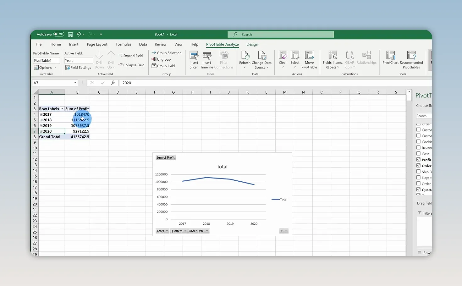
Power Query reads the folder again, includes the additional workbook, and applies the saved transformations. The loaded table now includes the 2020 records, and the analysis can include the new year.

Adding a file and refreshing are separate actions. In this workflow, the update happens when you run Refresh All. You aren’t setting up a live folder monitor.

That’s the real value of Power Query: it doesn’t just combine data once. It saves the process for getting and cleaning that data, so the next file becomes an update instead of another cleanup project. You can spend less time preparing spreadsheets and more time figuring out what the numbers mean.

Made with VideoToBlog using How to use Microsoft Power Query