You have a list of cookies, a price list, and a bunch of blank cells to fill in. You could look up each cookie and type its price manually, but hey, we have better things to do. Like eat the cookies.
VLOOKUP lets Excel find a matching item in a list and return information from the same row. We’ll use it to fill in cookie prices, fix a common error when copying formulas, and make the lookup easier to maintain as the price list changes.
To follow along, open the practice workbook.
What You'll Learn
- VLOOKUP finds an item in a range’s first column and returns a value from the same row.
- Use FALSE as the final argument to request an exact match.
- Lock the source range with absolute references to prevent it shifting when formulas are copied.
- Reference an Excel table to keep the lookup range aligned with a changing source list.
What Does VLOOKUP Do?
VLOOKUP stands for vertical lookup. It searches down the first column of a selected range for a value, then returns a value from another column in that same row.
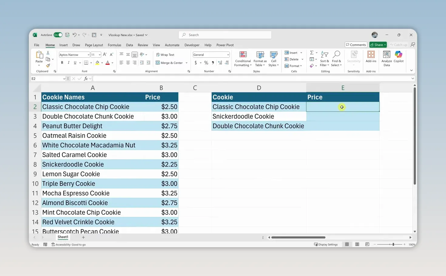
In our example, the source list on the left contains cookie names in column A and prices in column B. On the right, column D contains three cookies whose prices we need:
- Classic Chocolate Chip Cookie
- Snickerdoodle Cookie
- Double Chocolate Chunk Cookie
Classic chocolate chip happens to be my favorite. Its price is $2.50, but instead of typing that price into column E, we’ll have Excel retrieve it.
1. Start the VLOOKUP Formula
Click the first blank price cell, E2. Start by typing an equal sign, which tells Excel that you’re entering a formula. Then type the function name and an opening parenthesis:
=VLOOKUP(Excel displays a hint showing the arguments the function accepts. Here’s the full structure:
=VLOOKUP(lookup_value, table_array, col_index_num, [range_lookup])Those names might look a little intimidating, but each one answers a straightforward question:
- lookup_value: What are we trying to find?
- table_array: Where should Excel search?
- col_index_num: Which column contains the answer?
- range_lookup: Should Excel use an approximate match or an exact match?
2. Select the Lookup Value
The first argument is the item we want to find. In this case, that’s the Classic Chocolate Chip Cookie in D2.
While editing the formula, click D2. Excel inserts the cell reference for you. Then type a comma to move to the next argument:
=VLOOKUP(D2,We’re referring to the cell containing the cookie name rather than typing the name into the formula. That becomes especially useful when we copy the formula to the other cookies.
3. Select the Table Array
The table array is the range Excel will search. It needs to include both the cookie names and the prices, because Excel needs the names to find a match and the prices to return an answer.
Select the source data in A2:B16, then enter another comma:
=VLOOKUP(D2,A2:B16,At this point, we’ve told Excel to look for the value in D2 within the first column of A2:B16.
4. Enter the Column Index Number
Next comes the column index number. What the heck is that? It’s simply the position of the column containing the value we want back, counted from the left edge of the selected range.
- The cookie names are in the first column of our range.
- The prices are in the second column.
We want the price, so enter 2, followed by a comma:
=VLOOKUP(D2,A2:B16,2,Count columns within the selected range, not across the entire worksheet. The leftmost column in the table array is column 1.
5. Choose an Exact Match
The last argument tells Excel whether to use an approximate match or an exact match. Here, we want to find the cookie name exactly, so choose FALSE.
You can type FALSE or select it from Excel’s suggestion list. Close the parenthesis and press Enter:
=VLOOKUP(D2,A2:B16,2,FALSE)Excel returns 2.5, which is $2.50. Not bad for such a delicious cookie.
For this kind of named-item lookup, explicitly using FALSE makes the matching choice clear. Microsoft’s VLOOKUP function reference provides additional details about the arguments.
Use the Function Helper If You Need a Hand
You don’t have to remember every argument while typing. With the formula selected, click the fx icon next to the formula bar to open Excel’s function helper.
The dialog gives each argument its own field. Click into a field to see an explanation of what belongs there. You can also see previews of the values being supplied and the formula’s result.
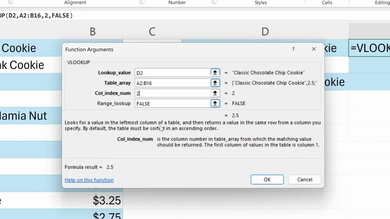
This is particularly helpful when you know what you want Excel to do but aren’t quite sure which argument goes where.
6. Copy the Formula Down and Check for Errors
We have one price, but we still need prices for snickerdoodle and double chocolate chunk. Use the fill handle at the bottom-right corner of E2 to copy the formula down through E4.
There’s a problem: the double chocolate chunk lookup returns #N/A.
Click into that formula and inspect its range. Because we copied it down two rows, Excel also moved the source range down two rows:
=VLOOKUP(D4,A4:B18,2,FALSE)The original source range was A2:B16. Now it’s A4:B18, which leaves out the Double Chocolate Chunk Cookie near the top of the source list. Excel can’t find it because the formula is no longer searching the full list.
This happens because A2:B16 is a relative reference. Relative references adjust when you copy a formula.
That adjustment is useful for the lookup value: D2 should become D3 and then D4 so each row searches for its own cookie. But we don’t want the source list moving along with it.
7. Lock the Source Range with Absolute References
To keep the lookup range fixed, turn it into an absolute reference.
- Select E2 and edit the formula.
- Select the A2 reference within the formula and press F4 to add dollar signs before the column and row.
- Do the same for B16, so both ends of the range are locked.
- Press Enter, then copy the corrected formula down again.
You can also type the dollar signs yourself. The corrected formula is:
=VLOOKUP(D2,$A$2:$B$16,2,FALSE)Now, when you copy it down to the double chocolate chunk row, it becomes:
=VLOOKUP(D4,$A$2:$B$16,2,FALSE)The cookie reference changes, but the price-list reference stays fixed. That’s exactly what we want.
The results now match the source list:
- Classic Chocolate Chip Cookie: $2.50
- Snickerdoodle Cookie: $2.25
- Double Chocolate Chunk Cookie: $3.00
8. Make the Lookup Easier to Maintain with an Excel Table
Absolute references solve the copying problem, but a fixed range still needs attention when your list changes. For example, new cookies added below the referenced range may not be included in the lookup.
A better approach for a changing list is to convert the source data into an Excel table.
- Click a cell inside the source cookie-and-price list.
- Open the Insert tab and select Table.
- Confirm the selected range includes the source list and its headings.
- Check My table has headers, then click OK.
Next, edit the VLOOKUP formula. Remove the absolute range reference, then select the whole source table instead.
In this workbook, Excel names the table Table6, and selecting the entire table produces the reference Table6[#All]. The formula becomes:
=VLOOKUP(D2,Table6[#All],2,FALSE)Your table name may be different. Use the reference Excel inserts when you select your table.
Press Enter and copy the formula down. The prices still come back correctly, but now the lookup points to the table rather than a fixed set of cell addresses. As you add or remove entries within that table, the reference follows the table’s size.
The VLOOKUP Pattern to Remember
A VLOOKUP formula needs four decisions: what to find, where to search, which column to return, and how to match. For our cookie price list, that means the cookie-name cell, the source list, column 2, and FALSE for an exact match.
When you copy the formula, let the lookup value change for each row, but keep the source list stable with absolute references or an Excel table. That’s the difference between a formula that works once and one you can reuse across the whole list.
And why did VLOOKUP break up with its data table? It couldn’t find a match. Okay, that one was bad.
Made with VideoToBlog using VLOOKUP in Excel | Step-by-Step Tutorial for Beginners


