How to Build an Interactive Dashboard in Excel

An interactive Excel dashboard brings your most important business information together on one sheet. Instead of digging through rows of sales data, you can compare markets, track monthly performance, and filter the results with a few clicks.

Best of all, you don’t need VBA or any add-ins. We’ll use tools built into Microsoft Excel: tables, PivotTables, PivotCharts, slicers, and a timeline. When new data arrives, you can add it to the source table and refresh the dashboard without rebuilding everything.

For this example, I’m creating a performance dashboard for the Kevin Cookie Company. Leadership keeps asking about profit and unit sales, so we’ll give them a dashboard that answers those questions. That leaves a little more time for making technology tutorials. And cookies, of course.

You can follow along with the sample Excel workbook.

Table of Contents

• 1. Plan the Dashboard Around Three Useful Views
• 2. Convert the Source Data into an Excel Table
• 3. Create Three Supporting PivotTables
• 4. Build the Profit by Market and Cookie Type Chart
• 5. Add Monthly Unit Sales and Profit Charts
• 6. Align and Size the Dashboard Charts
• 7. Add a Timeline and Slicers
• 8. Add New Data and Refresh the Dashboard
• 9. Polish the Appearance and Share the Workbook

1. Plan the Dashboard Around Three Useful Views

Before building charts, decide what questions the dashboard should answer. Our dashboard will contain three views:

• Profit by market and cookie type: Which countries generate the most profit, and which products contribute to it?
• Units sold each month: How does sales volume change over time?
• Profit by month: How does profitability change over time?

We’ll also add controls for date, country, and product. Those filters will work across all three charts, so someone can select a market or cookie type and immediately see the related performance.

The workbook’s Data worksheet contains sales records with fields such as Country, Product, Units Sold, Revenue, Cost, Profit, and Date. This tabular layout works well for PivotTables: each column represents a field, and the header row identifies those fields.

Keep a separate Dashboard worksheet for the finished visuals. The source data and supporting PivotTables can stay on their own sheets.

2. Convert the Source Data into an Excel Table

The first step is important for keeping the dashboard easy to update. Data arranged in rows and columns is not necessarily an actual Excel table. We need to turn it into one.

1. Open the Data worksheet and click any cell within the dataset.
2. Select Insert > Table, or press Ctrl + T.
3. Check that Excel has selected the full data range.
4. Select My table has headers.
5. Click OK.

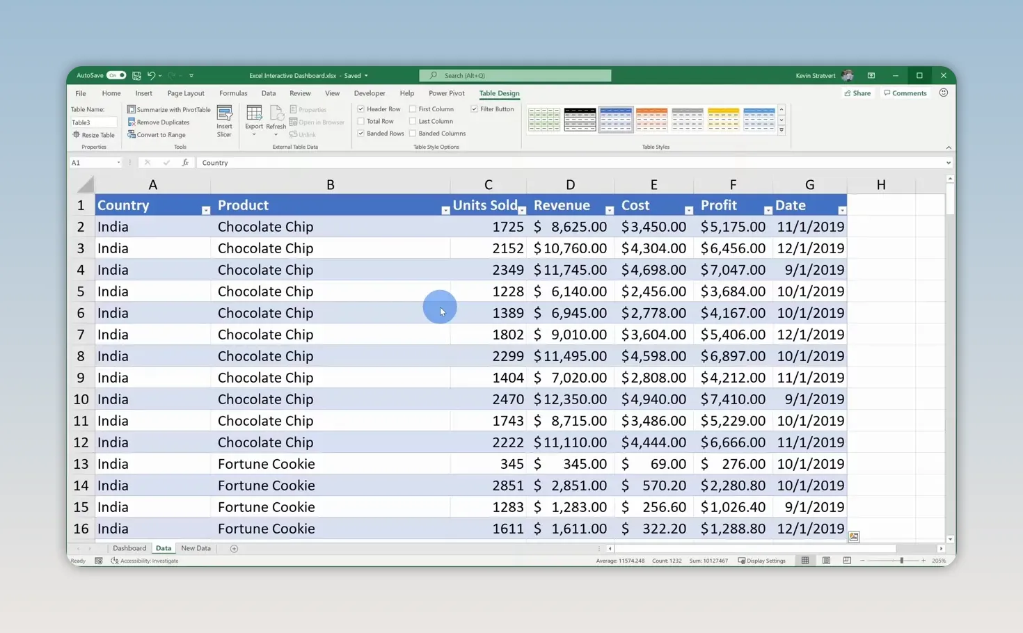
Excel applies table formatting and adds filter buttons to the headers. The formatting is nice, but the real benefit comes later: when you append new records directly below the table, the table expands to include them.

By building our PivotTables from this table rather than a fixed cell range, we won’t have to manually extend the source range each time new sales data arrives.

3. Create Three Supporting PivotTables

Each chart in this dashboard will have its own PivotTable. The PivotTables summarize the data, and the PivotCharts turn those summaries into visuals.

1. Click inside the Excel table.
2. Select Insert > PivotTable.
3. Confirm that the table is selected as the source. In the sample, Excel assigns it a name such as Table3.
4. Choose New Worksheet and click OK.

You’ll now have an empty PivotTable and the PivotTable Fields pane.

Rather than repeating the insertion process twice, duplicate this worksheet. Hold Ctrl, click its sheet tab, and drag the tab to another position. Repeat that once more. You now have three sheets containing PivotTables based on the same source.

Rename the sheets to make their purposes clear:

• Profit by country and cookie
• Units sold each month
• Profit by month

If PivotTables are new to you, my introduction to PivotTables provides more background. There’s also an advanced PivotTables tutorial for exploring additional features. There’s always something new to learn with these.

4. Build the Profit by Market and Cookie Type Chart

Arrange the PivotTable fields

On the first supporting sheet, drag the fields into these areas:

• Rows: Country
• Columns: Product
• Values: Profit, summarized as a sum

This gives you a breakdown of profit for each country and cookie type, along with grand totals.

Select the numeric values, go to Home, and apply Currency formatting. Reduce the decimal places to zero. Every penny counts, but we don’t need every penny displayed in this analysis.

Sort the results by profitability

A ranked chart is easier to read than one arranged alphabetically. Sort both the markets and the cookie types by their total profit.

1. Right-click a country’s value in the Grand Total column.
2. Select Sort > Sort Largest to Smallest.
3. Right-click a product total in the bottom Grand Total row.
4. Again, select Sort > Sort Largest to Smallest.

In the initial sample data, India is the most profitable market and the United States is the least profitable. Sorting makes that comparison much easier to spot.

Insert and clean up the PivotChart

1. Click inside the PivotTable.
2. Select PivotTable Analyze > PivotChart.
3. Choose Column > Stacked Column and click OK.
4. On the chart’s Design tab, select Add Chart Element > Chart Title > Above Chart.
5. Enter Profit by Market & Cookie Type.

The stacked column chart shows total profit by market while also showing each cookie type’s contribution. Because we sorted the PivotTable, the markets run from highest total profit on the left to lowest on the right. The product order also places the largest overall contributor at the bottom of the stacks.

PivotCharts include field buttons for filtering, but we’ll use slicers instead. Right-click one of those buttons and choose Hide All Field Buttons on Chart.

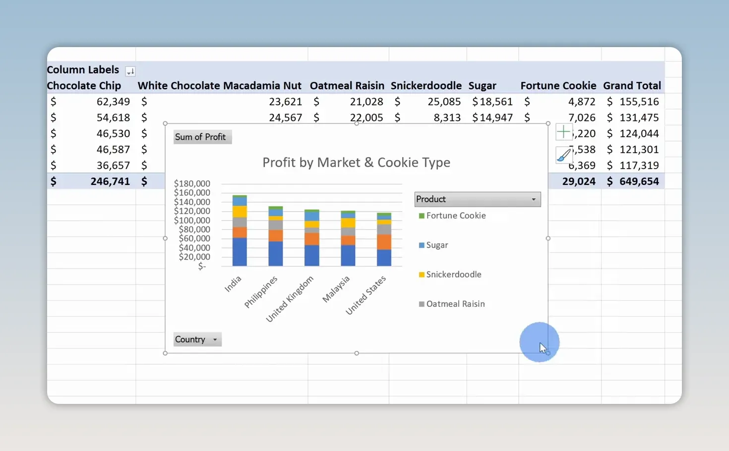
Select the chart’s border, press Ctrl + C, open the Dashboard sheet, and press Ctrl + V. Position this chart toward the middle-left, leaving room for filters along the far left and two line charts on the right.

5. Add Monthly Unit Sales and Profit Charts

Create the units sold chart

Open the Units sold each month sheet and arrange the fields as follows:

• Rows: Date, displayed at the month level
• Values: Sum of Units Sold

In this example, Excel groups the dates into months. If your dates remain as individual days, group the date field by months before continuing.

Select the sales totals, apply Comma Style from the Home tab, and remove the decimal places. This keeps large unit counts readable without suggesting that we sold part of a cookie.

1. Select PivotTable Analyze > PivotChart.
2. Choose a Line chart and click OK.
3. Change the chart title to Units sold each month.
4. Select the single-series legend and delete it.
5. Right-click a field button and select Hide All Field Buttons on Chart.
6. Copy the chart and paste it onto the upper-right area of the Dashboard sheet.

A line chart works well here because the main question is how sales change over time. With only one series, the chart title already explains what the line represents, so the legend doesn’t add much.

Create the profit by month chart

On the Profit by month sheet, use a similar setup:

• Rows: Months from the Date field
• Values: Sum of Profit

Format the profit totals as currency with no decimal places. Insert another line PivotChart, then clean it up:

1. Set the title to Profit by month.
2. Delete the legend labeled Total.
3. Hide all chart field buttons.
4. Copy the chart to the Dashboard sheet and place it below the units sold chart.

The initial data shows profit declining in November and December. Those are the holidays, so I’d expect the cookie business to be doing very well. That’s exactly the kind of result management may want to investigate. The chart highlights the pattern, even though it doesn’t explain the cause.

6. Align and Size the Dashboard Charts

A dashboard becomes much easier to read when the objects line up. You don’t have to get everything right by dragging freehand.

• Snap objects to cells: Hold Alt while moving or resizing a chart to snap its edges to worksheet cell boundaries.
• Align chart edges: Select multiple chart objects and use Shape Format > Align. Align the stacked column chart and upper line chart to the top, then align the two line charts to the left.
• Set exact dimensions: Select a chart and use the height and width controls on the Format tab to give related charts matching dimensions.

For this layout, the stacked column chart occupies the taller central area, while the two equally sized line charts sit one above the other on the right. The remaining space on the left will hold the interactive controls.

7. Add a Timeline and Slicers

At this point, the dashboard looks useful, but it’s still static. A timeline and slicers let people change the data shown without opening the supporting PivotTables.

Insert a date timeline

1. Select a PivotChart on the Dashboard sheet.
2. Open PivotChart Analyze > Insert Timeline.
3. Select Date and click OK.
4. Move the timeline to the upper-left area of the dashboard.
5. Resize it to fit the space reserved for filters.

The timeline provides a visual date filter, with months shown in this example.

Insert country and product slicers

1. Select a PivotChart again.
2. Choose PivotChart Analyze > Insert Slicer.
3. Select Country and Product.
4. Click OK.

Move the two slicers below the timeline. Resize them so their buttons fit without unnecessary empty space.

You can also simplify their appearance. If the country and product names make the purpose obvious, right-click each slicer, select Slicer Settings, and clear Display header.

To make the filter area look consistent, give the timeline and both slicers the same width using their ribbon size controls. In this example, I use a width of 2 inches for each.

Connect every filter to every PivotTable

This is the step that makes the dashboard work as one connected report. Initially, selecting India in the country slicer may update only the market profit chart. The other two charts stay unchanged because the slicer isn’t connected to their PivotTables yet.

1. Right-click the country slicer.
2. Select Report Connections.
3. Check all three supporting PivotTables.
4. Click OK.
5. Repeat the connection setup for the product slicer and the date timeline.

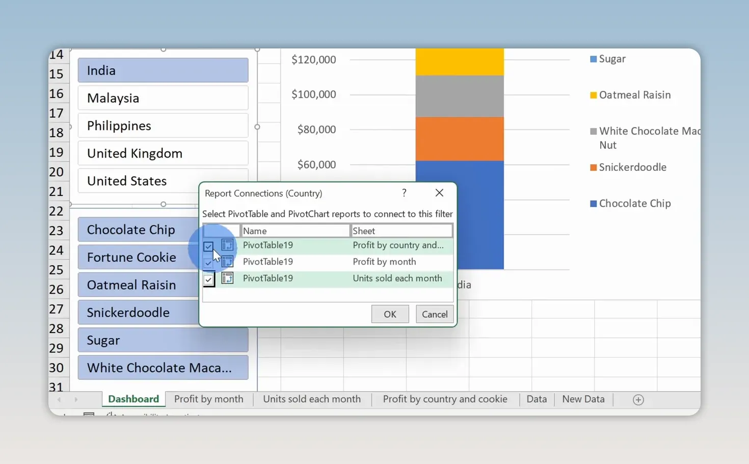
Now test the dashboard. Select United States and Chocolate Chip. All three charts should show results for that country and product combination.

You can also select multiple adjacent slicer items by clicking and dragging across the buttons. For example, select several countries to compare their profit while keeping the same product selection. The monthly charts update to reflect those selections too.

8. Add New Data and Refresh the Dashboard

The sample workbook includes a New Data worksheet with additional records for 2020. These records use the same column structure as the original data.

1. Open New Data and copy the new data rows, without repeating the header row.
2. Open the original Data sheet.
3. Paste the records directly beneath the last row of the source table.
4. Confirm that the table expands to include the new rows.
5. Return to the Dashboard sheet and select a PivotChart.
6. Choose PivotChart Analyze > Refresh > Refresh All.

The PivotTables and charts now incorporate the expanded dataset.

The table expands automatically, but the PivotTables still need to be refreshed. Those are two separate parts of the update process. Converting the source data into a table saves you from redefining its range; Refresh All brings those new records into the dashboard.

9. Polish the Appearance and Share the Workbook

Make the sheet look more like a dashboard

With the Dashboard sheet active, open the View tab and turn off:

• Gridlines, to remove the worksheet’s cell grid.
• Headings, to remove the row numbers and column letters.

Next, select the supporting worksheets containing the data and PivotTables, right-click their tabs, and choose Hide. Leave the Dashboard sheet visible so it’s the main entry point to the workbook.

Apply a theme

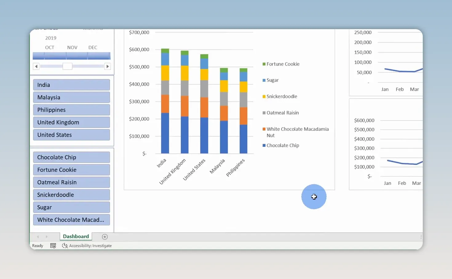
If the default colors don’t match your organization, open Page Layout > Themes and choose a different theme. This changes the dashboard’s theme-based styling, including the chart colors.

You can browse for additional themes or save a theme you’ve customized. That makes it easier to give the dashboard the look you want without individually recoloring every visual.

Choose sharing permissions

When you’re ready to distribute the workbook, click Share in Excel’s upper-right corner.

1. Open the sharing or link settings.
2. Decide whether recipients should be able to edit or have view-only access.
3. Enter the people you want to share with, or select Copy Link to distribute a link.

For additional help with the commands available in your edition, use Microsoft’s Excel help and learning resources.

You now have an interactive Excel dashboard with ranked profit comparisons, monthly performance trends, and shared filters. As new sales records arrive, append them to the source table and refresh. The same dashboard keeps answering the business questions, without requiring VBA, add-ins, or a fresh set of charts every month.

Made with VideoToBlog using 📊 How to Build Excel Interactive Dashboards